Julia 可视化库:VegaLite.jl 【笔记4 - 数据来源】
内部数据来源
Julia 表格数据结构
VegaLite.jl 涵盖了 julia 生态系统中的大多数表格数据结构: DataFrames.jl,JuliaDB.jl,IndexedTables.jl,各种文件IO库(CSVFiles.jl,FeatherFiles.jl,ExcelFiles.jl,StatFiles.jl,ParquetFiles.jl)以及 Query.jl 中的表格形式。
管道操作数据
using VegaLite, VegaDatasets, Query
cars = dataset("cars");
cars |>
@vlplot(
    :point,
    x=:Horsepower,
    y=:Miles_per_Gallon
)
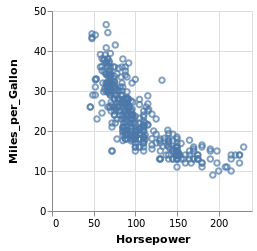
上面的写法等价于 @vlplot(:point, data=cars, x=“Horsepower:q”, y=“Miles_per_Gallon:q”)
cars |> # 绘制日本地区的情况
    @filter(_.Origin=="Japan") |>
    @vlplot(
    :point,
    x={:Horsepower, scale={zero=false}},
    y=:Miles_per_Gallon)
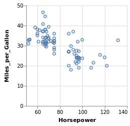
# 上面的写法等价于
cars |>
    @vlplot(
    :point,
    transform=[{filter="datum.Origin == 'Japan'"}],
    x={:Horsepower, scale={zero=false}},
    y=:Miles_per_Gallon)
外部数据来源
主要是从 本地文件路径 和 网络 获得数据。这一部分功能目前还不完善。
参见:http://fredo-dedup.github.io/VegaLite.jl/stable/userguide/data.html#Referencing-external-data-1
using FilePaths
# path = p"folder/filename.csv";
# path |> @vlplot(:point, x=:a, y=:b)
上面的命令运行报错,估计功能还没实现。推荐将数据读取进来,然后进行管道操作 ↓
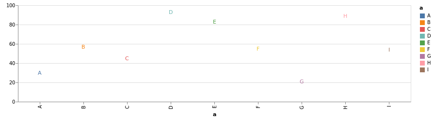
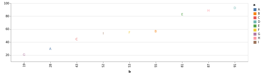
using CSV
data = CSV.read("data/data.csv") # 笔记 3 中的数据
| a | b | |
|---|---|---|
| 1 | A | 28 |
| 2 | B | 55 |
| 3 | C | 43 |
| 4 | D | 91 |
| 5 | E | 81 |
| 6 | F | 53 |
| 7 | G | 19 |
| 8 | H | 87 |
| 9 | I | 52 |
data |> @vlplot(:text, x={:a, scale={zers=false}}, y={:b, title=nothing}, text=:a, color=:a)
data |> @vlplot(:text, x="b:o", y={:b, title=nothing, scale={zero=false}}, text=:a, color=:a)
Julia 可视化库:VegaLite.jl 【笔记5 - 绘图类型 mark】
Galary & API
VegaLite.jl 文档绘图例子: http://fredo-dedup.github.io/VegaLite.jl/stable/index.html
VegaLite 官方 Example Galary: Example Gallery | Vega-Lite
VegaLite API 文档( JSON 格式): Overview | Vega-Lite
mark 特性
// Json 版本
{
  ...
  "mark": {
    "type": ...,       // mark
    ...
  },
  ...
}
# Julia 版本
@vlplot(
    mark={
        typ=:..., # 注意不能使用 Julia 预留关键字 type
        ...
    }
)
狭义的 mark 指的是 mark 键下的 type 字段
| 类型 | mark → type | x | y | color | shape | size |
|---|---|---|---|---|---|---|
| 线图 | :line | |||||
| 轨迹图 | :trace | |||||
| 垂线、水平线图 | :rule | |||||
| 空心散点图 | :point | |||||
| 圆形实心散点图 | :circle | |||||
| 方形实心散点图 | :square | |||||
| 文字标注图 | :text | text=:var | ||||
| 柱状图 | :bar | |||||
| 直方图 | :bar | x={:a, bin=true} | y=“count()” | |||
| 热力图、填充图 | :rect | x=“x:o” | y=“y:o” | color=:z | ||
| area plot (面积堆积图) | :area | |||||
| strip plot(分布散点图) | :tick | x=:x | y=“y:o” | |||
| 地理图 | :geoshape |
广义的 mark 包括:type、 style、 clip 三部分。
详细 mark 特性参看: Mark | Vega-Lite
几个栗子
运行例子代码前需要加载以下库 ↓
using VegaLite, VegaDatasets
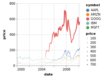
Example1
dataset("stocks") |>
@vlplot(
    :trail, # 等价于 mark = :trail 等价于 mark={typ=:trail}
    x={
        "date:t",
        axis={format="%Y"}
    },
    y=:price,
    size=:price,
    color=:symbol
)
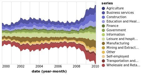
Example2
dataset("unemployment-across-industries") |>
@vlplot(
    :area, # 等价于 mark = :area 等价于 mark={typ=:area}
    width=300, height=200,
    x={
        "yearmonth(date)",
        axis={
            domain=false,
            format="%Y",
            tickSize=0
        }
    },
    y={
        "sum(count)",
        axis=nothing,
        stack=:center
    },
    color={
        :series,
        scale={scheme="category20b"}
    }
)
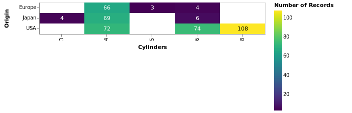
Example3
cars |>
    @vlplot(
        y="Origin:o",
        x="Cylinders:o",
        config={
            scale={bandPaddingInner=0, bandPaddingOuter=0},
            text={baseline=:middle}
        }
    ) +
    @vlplot(
        :rect, # 等价于 mark = :rect 等价于 mark={typ=:rect}
        color="count()") +
    @vlplot(
        :text, # 等价于 mark = :text 等价于 mark={typ=:text}
        text="count()",
        color={
            condition={
                test="datum['count_*'] > 100",
                value=:black
            },
            value=:white
        }
)
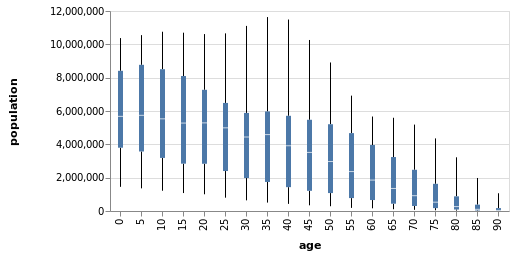
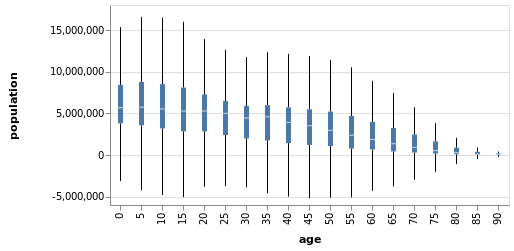
Example4
dataset("population") |>
@vlplot(
    transform=[{
        aggregate=[
            {op=:q1, field=:people, as=:lowerBox},
            {op=:q3, field=:people, as=:upperBox},
            {op=:median, field=:people, as=:midBox},
            {op=:min, field=:people, as=:lowerWhisker},
            {op=:max, field=:people, as=:upperWhisker}
        ],
        groupby=[:age]
    }]
) +
@vlplot(
    mark={:rule, style=:boxWhisker},
    y={"lowerWhisker:q", axis={title="population"}},
    y2="lowerBox:q",
    x="age:o"
) +
@vlplot(
    mark={:rule, style=:boxWhisker},
    y="upperBox:q",
    y2="upperWhisker:q",
    x="age:o"
) +
@vlplot(
    mark={:bar, style=:box},
    y="lowerBox:q",
    y2="upperBox:q",
    x="age:o",
    size={value=5}
) +
@vlplot(
    mark={:tick, style=:boxMid},
    y="midBox:q",
    x="age:o",
    color={value=:white},
    size={value=5}
)
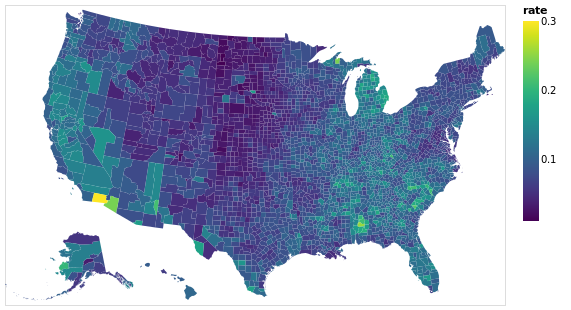
Example5
us10m = dataset("us-10m").path
unemployment = dataset("unemployment.tsv").path

p = @vlplot(
    :geoshape, # mark
    width=500, height=300,
    data={
        url=us10m,
        format={
            typ=:topojson,
            feature=:counties
        }
    },
    transform=[{
        lookup=:id,
        from={
            data=unemployment,
            key=:id,
            fields=["rate"]
        }
    }],
    projection={
        typ=:albersUsa
    },
    color="rate:q"
)
Julia 可视化库:VegaLite.jl 【笔记6 - transform 之 aggregate】
aggregate 特性
// Json 版本
{
  ...
  "transform": [
    {
      // Aggregate Transform
      "aggregate": [
          {"op": ..., "field": ..., "as": ...},
          {"op": ..., "field": ..., "as": ...},
          ...],
      "groupby": [...]
    }
     ...
  ],
  ...
}
# Julia 版本
@vlplot(
    ...
    transform=[{
        aggregate=[
            {op=..., field=..., as=...},
            {op=..., field=..., as=...},
            ...],
        groupby=[...]
        },
        ...
    ],
    ...
)
-
aggregate字段下有op、field、as三个必需的属性。-
field指的是操作的变量对象。 -
as给操作后的变量一个名称,该名称于所在的代码环境内起作用。 -
op支持以下操作函数。在Json格式中函数名称使用双引号,即使用"op": "operation",在Julia中语法为op=:operation。
-
-
aggregate可与groupby字段连用,实现对不同的组进行操作。
| operation | 解释 | operation | 解释 |
|---|---|---|---|
| count | 计数 | stderr | 标准误 |
| valid | 对非空等数值计数 | median | 中位数 |
| missing | 空值或未定义字段值 | q1 | 下四分位数 |
| distinct | 对不同字段的值计数 | q3 | 上四分位数 |
| sum | 求和 | ci0 | 根据bootstrapped方法得到的95%下置信区间 |
| mean | 均值 | ci1 | 根据bootstrapped方法得到的95%上置信区间 |
| average | 均值 | min | 最小值 |
| variance | 样本方差 | max | 最大值 |
| variancep | 总体方差 | argmin | 达到最小值的数据对象 |
| stdev | 样本标准差 | argmax | 达到最大值的数据对象 |
| stdevp | 总体标准差 |
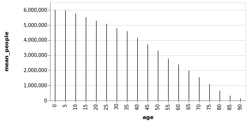
栗子
一个简单的例子:画出 poplulation 数据集中 150 年各年龄段的平均人口数量。
using VegaLite, VegaDatasets, DataFrames
popu = DataFrame(dataset("population"))
describe(popu[:,1]) # 1850-2000 年 -> 151 年
dataset("population") |>
@vlplot(
    transform=[
        {
            aggregate=[
            {op=:mean, field=:people, as=:mean_people} # 每个年龄段的人口均值
        ],
            groupby=[:age] # 以年龄段分组
        }
    ],
    :rule,
    x="age:o",
    y="mean_people:q",
)
Summary Stats:
Mean:           1927.333333
Minimum:        1850.000000
1st Quartile:   1880.000000
Median:         1930.000000
3rd Quartile:   1970.000000
Maximum:        2000.000000
Length:         570
Type:           Int64
应用
一个带有最大值、最小值触须的箱线图 ↓
using VegaLite, VegaDatasets
dataset("population") |>
@vlplot(
    transform=[{
        aggregate=[
            {op=:q1, field=:people, as=:lowerBox},
            {op=:q3, field=:people, as=:upperBox},
            {op=:median, field=:people, as=:midBox},
            {op=:min, field=:people, as=:lowerWhisker},
            {op=:max, field=:people, as=:upperWhisker}
        ],
        groupby=[:age]
    }]
) +
@vlplot(
    mark={:rule, style=:boxWhisker},
    y={"lowerWhisker:q", axis={title="population"}},
    y2="lowerBox:q",
    x="age:o"
) +
@vlplot(
    mark={:rule, style=:boxWhisker},
    y="upperBox:q",
    y2="upperWhisker:q",
    x="age:o"
) +
@vlplot(
    mark={:bar, style=:box},
    y="lowerBox:q",
    y2="upperBox:q",
    x="age:o",
    size={value=5}
) +
@vlplot(
    mark={:tick, style=:boxMid},
    y="midBox:q",
    x="age:o",
    color={value=:white},
    size={value=5}
)
Julia 可视化库:VegaLite.jl 【笔记7 - transform 之 calculate】
calculate 特性
// Json 版本
{
  ...
  "transform": [
      // Calculate Transform
      {"calculate": ..., "as" ...},
      {"calculate": ..., "as" ...},
      {"filter": ...},
       ...
  ],
  ...
}
# Julia 版本
@vlplot(
    ...
    transform=[
        {calculate= ..., as= ...},
        {calculate= ..., as= ...},
        {filter= ...},
        ...
    ],
    ...
)
-
calculate的值为expression表达式,datum表示当前输入的数据对象,datum.a表示对输入数据列名为 a 的数据进行计算。 -
expression中默认的常量有: NaN、 E (常数 e )、LN2 ($log_e 2$)、LN10 ($log_e 10$)、LOG2E ($log_2 e$)、LOG10E ($log_{10} e$)、MAX_VALUE (可表示的最大正数)、MIN_VALUE (可表示的最小正数)、PI ($\pi$)、SQRT1_2($\sqrt {1/2})、*SQRT2* (\sqrt 2$)等。 -
calculate可与filter连用,对满足某些条件的数据进行计算操作。
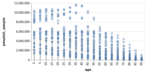
栗子
使用 LOG10E 常量,以历史上各年龄段人口数量顶峰值与这个常量的乘积作为y轴,作出垂直线图。并将各年龄段的历史人口数情况以散点形式添加到图上。
using VegaLite, VegaDatasets
dataset("population") |>
@vlplot() + # 这里相当于定义一层 layer,"+" 表示添加图层
@vlplot(
    transform=[
        {
            calculate="LOG10E * datum.people",
            # 相当于 log(10, e) * max(people), log(10, e) ≈ 0.434
            as=:people2
        }
    ],
    :rule,
    x="age:o",
    y="people2:q",
)+
@vlplot(
    :point,
    x="age:o",
    y="people:q"
)
应用
带有 1.5 倍四分位距的箱线图 ↓
using VegaLite, VegaDatasets
dataset("population") |>
@vlplot(
    transform=[
        {
            aggregate=[
                {op=:q1, field=:people, as=:lowerBox},
                {op=:q3, field=:people, as=:upperBox},
                {op=:median, field=:people, as=:midBox}
            ],
            groupby=[:age]
        },
        {
            calculate="datum.upperBox - datum.lowerBox",
            as=:IQR
        },
        {
            calculate="datum.lowerBox - datum.IQR * 1.5",
            as=:lowerWhisker
        },
        {
            calculate="datum.upperBox + datum.IQR * 1.5",
            as=:upperWhisker
        }
    ]
) +
@vlplot(
    mark={:rule, style=:boxWhisker},
    y={"lowerWhisker:q", axis={title="population"}},
    y2="lowerBox:q",
    x="age:o"
) +
@vlplot(
    mark={:rule, style=:boxWhisker},
    y="upperBox:q",
    y2="upperWhisker:q",
    x="age:o"
) +
@vlplot(
    mark={:bar, style=:box},
    y="lowerBox:q",
    y2="upperBox:q",
    x="age:o",
    size={value=5}
) +
@vlplot(
    mark={:tick, style=:boxMid},
    y="midBox:q",
    x="age:o",
    color={value=:white},
    size={value=5}
)
Julia 可视化库:VegaLite.jl 【笔记8 - transform 之 filter】
filter 特性
// Json 版本
{
  ...
  "transform": [
      // Filter Transform
      {"filter": ...}
     ...
  ],
  ...
}
# Julia 版本
@vlplot(
    ...
    transform=[
        {filter= ...},
        ...
    ],
    ...
)
filter 的值为逻辑值有以下四种情况:
-
表达式字符串,以
datum标示当前输入数据对象。如filter="datum.a > 60"表示筛选出数据中字段为 a ,其值大于 60 的整个数据对象。 -
包含以下字段谓语: equal (等于), lt (小于), lte (小于等于), gt (大于), gte (大于等于), range (表示数值或者时间范围), oneOf (表示属于某个集合)。
如 filter={field=:car_color, equal=“red”}} 表示筛选 car_color 为 red 的数据对象; filter={field=:car_color, oneOf=[“red”, “yellow”]}} 表示筛选 car_color 为 red 或者 yellow 的数据对象。
-
selection predicate。参见: Filter Transform | Vega-Lite
-
前三种情况的组合。
栗子
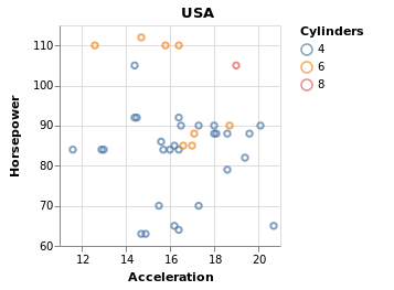
画出 cars 数据集中,1980年至1982年美国地区的汽车情况。
using VegaLite, VegaDatasets
dataset("cars") |>
@vlplot(
    transform=[
        {filter="datum.Origin=='USA'"},  # 注意字符串内层使用的单引号
        {filter={field=:Year, oneOf=["1980-01-01", "1981-01-01", "1982-01-01"]}},
    ],
    :point,
    x={:Acceleration, scale={zero=false}}, # 坐标范围不从 0 开始
    y={:Horsepower, scale={zero=false}},
    color="Cylinders:n",
    title="USA"
)
应用
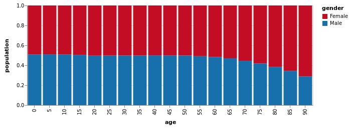
描绘20世纪世界人口各年龄段性别比例构成情况。
using VegaLite, VegaDatasets
dataset("population") |>
@vlplot(
    :bar,
    transform=[
        {filter={field=:year, range=[1900, 2000]}},
        {calculate="datum.sex==2 ? 'Female' : 'Male'",as="gender"}
    ],
    enc={
        y={
            "sum(people)",
            axis={title="population"},
            stack=:normalize # 归一化
        },
        x={
            "age:o",
            scale={rangeStep=30} # 调整柱子的宽度
        },
        color={
            "gender:n",
            scale={range=["#c30d24", "#1770ab"]}
        }
    }
)
完 ![]()