1. 一个例子
数据准备
X = (a = rand(12), b = rand(12), c = rand(12))
y = X.a .+ 2 .* X.b + 0.05 .* rand(12)
模型训练
model = @load RidgeRegressor pkg=MultivariateStats
[评估]单个measure
rng = StableRNG(1234)
cv = CV(nfolds = 3, shuffle = true) # 重采样策略
evaluate(model, X, y, resampling = cv, measure = l2)

# 也可以这样, 下面也是
mach = machine(model, X, y)
evaluate!(mach, resampling = cv, measure = l2)
| _.measure | _.measurement | _.per_fold |
|---|---|---|
| l2 | 0.164 | [0.105, 0.23, 0.158] |
_.per_observation = [[[0.288, 0.128, …, 0.186], [0.136, 0.534, …, 0.348], [0.435, 0.0345, …, 0.298]], missing, missing]
[评估] 多个measure
evaluate(model, X, y, resampling = cv, measure = [l1, rms, rmslp1])
| _.measure | _.measurement | _.per_fold |
|---|---|---|
| l1 | 0.35 | [0.505, 0.319, 0.226] |
| rms | 0.424 | [0.51, 0.454, 0.273] |
| rmslp1 | 0.197 | [0.193, 0.256, 0.116] |
_.per_observation = [[[0.61, 0.514, …, 0.414], [0.00912, 0.486, …, 0.0136], [0.139, 0.144, …, 0.491]], missing, missing]
来看看文档是怎么解释这些参数的
•   measure: the vector of specified measures

•   measurements: the corresponding measurements, aggregated across the
	test folds using the aggregation method defined for each measure
	(do aggregation(measure) to inspect)

•   per_fold: a vector of vectors of individual test fold evaluations
    (one vector per measure)

•   per_observation: a vector of vectors of individual observation
    evaluations of those measures for which
    reports_each_observation(measure) is true, which is otherwise
    reported missing.
在这里我们统一用evaluate!(machine)的规定
2. 评估模型的必要参数
2.1 resampling
内置重采样策略有三个, Holdout, CV 与 StratifiedCV
2.1.1 Holdout
其实就跟sklearn里的train_test_split差不多,将训练集和测试集按一定比例划分
holdout = Holdout(; fraction_train=0.7,
                   	shuffle=nothing,
					rng=nothing)
2.1.2.CV
交叉验证重采样策略
cv = CV(; nfolds=6, shuffle=nothing, rng=nothing)
2.1.3 StratifiedCV
分层交叉验证重采样策略,仅适用于分类问题(OrderedFactor或Multiclass目标)
stratified_cv = StratifiedCV(; nfolds=6,
                               shuffle=false,
                               rng=Random.GLOBAL_RNG)
2.2 measure
2.2.1 分类指标
- 混淆矩阵
| Ground | Truth | |
|---|---|---|
| Predicted | Positive | Negative |
| True | TP | FN |
| False | FP | TN |
-
由混淆矩阵推导出的概率
- 准确率
- 精确率
- 召回率
[补充] FScore为精确率与召回率的调和平均
我太懒了,别人比我总结的好,看这篇文章吧
2.2.2 回归指标
- l1
∑|(Yᵢ - h(xᵢ)| - l2
∑(Yᵢ - h(xᵢ))² - mae
平均绝对误差
l1(Ŷ,h(xᵢ)) / n - mse
平均平方误差
l2(Ŷ,h(xᵢ)) / n - rmse
均方根误差
√(∑(ŷ - y)²
ps: 不会用latex啊![]() ,函数我都写在w思维导图里了,详细文档看这里
,函数我都写在w思维导图里了,详细文档看这里
2.2.3 扩展包 LossFunction
TODO LossFunctions (外部包)查询
包介绍
The LossFunctions.jl package includes “distance loss” functions for Continuous targets, and “marginal loss” functions for Binary targets. While the LossFunctions,jl interface differs from the present one (for, example Binary observations must be +1 or -1), one can safely pass the loss functions defined there to any MLJ algorithm, which re-interprets it under the hood. Note that the “distance losses” in the package apply to deterministic predictions, while the “marginal losses” apply to probabilistic predictions.
github地址:
LossFunctions提供了更多的指标,拿文档里的代码举个例子
using LossFunctions

X = (x1=rand(5), x2=rand(5));
y = categorical(["y", "y", "y", "n", "y"]);
w = [1, 2, 1, 2, 3];

mach = machine(ConstantClassifier(), X, y);
holdout = Holdout(fraction_train=0.6);
evaluate!(mach,
          measure=[ZeroOneLoss(), L1HingeLoss(), L2HingeLoss(), SigmoidLoss()],
          resampling=holdout,
          operation=predict,
          weights=w)
| _.measure | _.measurements | _.per_fold |
|---|---|---|
| ZeroOneLoss | 0.4 | [0.4] |
| L1HingeLoss | 0.8 | [0.8] |
| L2HingeLoss | 1.6 | [1.6] |
| SigmoidLoss | 0.848 | [0.848] |
| _.per_observation = [[[0.8, 0.0]], [[1.6, 0.0]], [[3.2, 0.0]], [[1.409275324764612, 0.2860870128530822]]] |
2.3 weights
权重,无所谓了,必要的时候才设
3. 评估模型的图表
跟你们说一下,我好像问了很多菜鸟的问题,作者太忙没时间理我![]()
我怕时间耽搁太久,先发出来好了
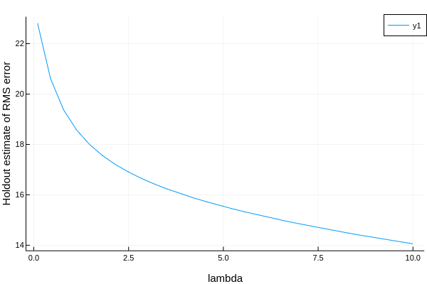
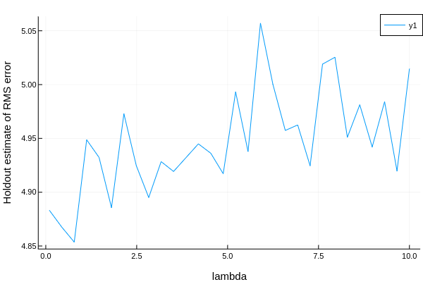
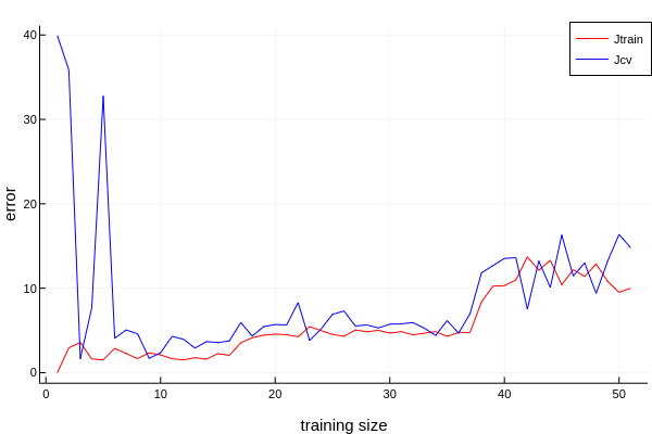
TODO 学习曲线
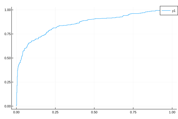
TODO ROC
TODO PR