[MLJ]数据处理

nesteiner · 2020 年7 月 24 日 13:04

思维导图做的太大了，我还是分开截图好了

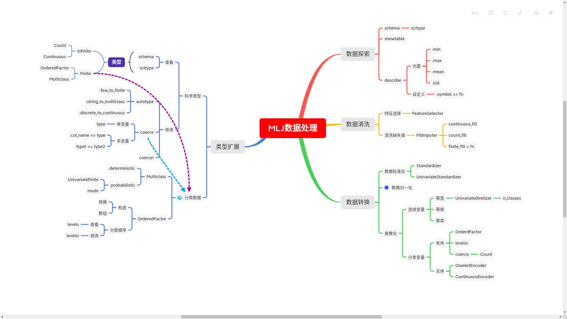
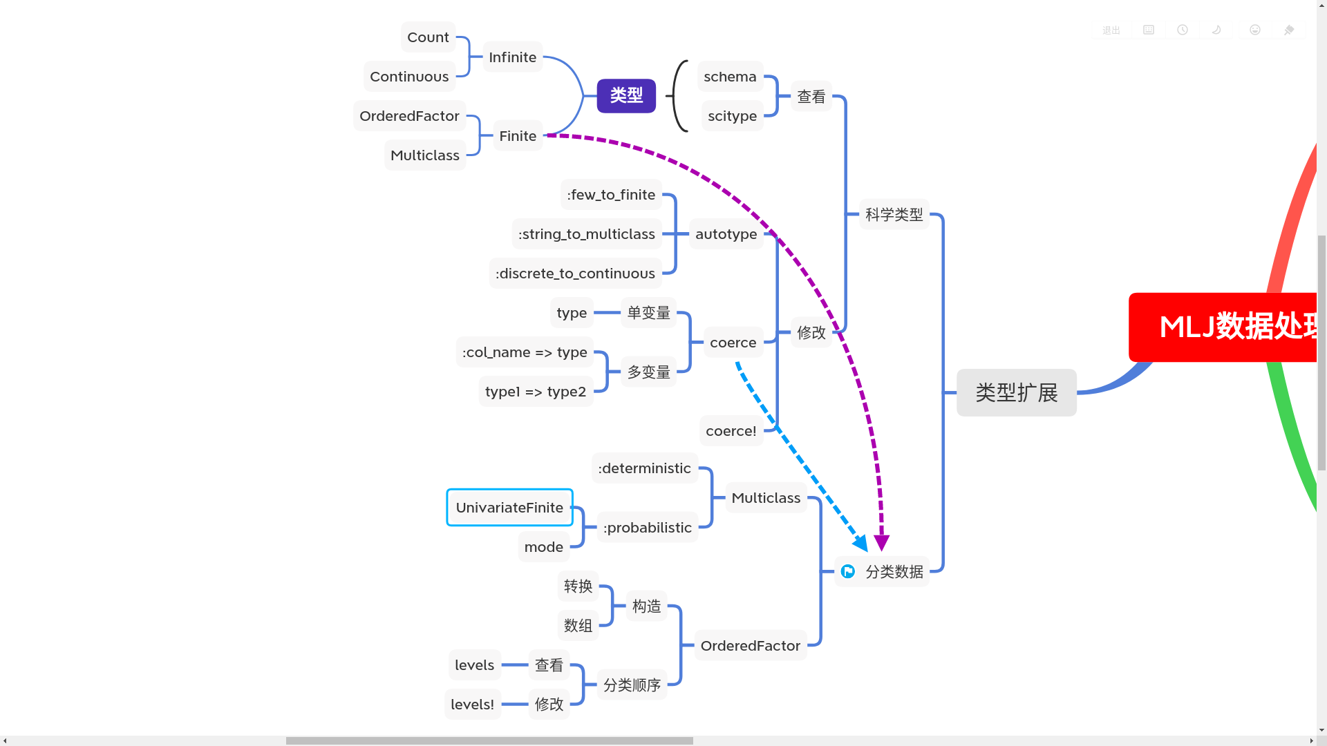
0. [非常重要] 类型扩展

我们先准备下数据，以波士顿房价为例，不过我们不用MLJ的@load_boston了，因为我们有许多工作需要DataFrame来完成

using MLJ
using TableView # for showtable

using RDatasets
boston = dataset("MASS", "Boston");
y, X = unpack(boston, col -> col == :MedV, col -> col != :MedV) # MedV 平均房价特征

tips
unpack拆包数据集，可以分别用函数指定需要的数据集

0.1 科学类型

0.1.1 科学类型介绍

MLJ扩展出了一系列类型来更好地解释数据集，这种类型叫做科学类型
科学类型还为模型和指标的搜索,查询提供了便利
模型

models(matching(X,y))
models(matching(X))

julia> info("RidgeRegressor", pkg="MLJLinearModels")
...
# 输入数据的科学类型
 input_scitype = Table{_s23} where _s23<:(AbstractArray{_s25,1} where _s25<:Continuous),
 # 输出数据的科学类型
 target_scitype = AbstractArray{Continuous,1},
...

指标

measures(matching(y))

julia> info(l1)
absolute deviations; aliases: `l1`.
...
# 虽然也是target，但这个其实是输入的数据类型
 target_scitype = Union{AbstractArray{Continuous,1}, AbstractArray{Count,1}},
...

0.1.2 查看科学类型

在数据分析中用到科学类型最多的类型有两种，一种是无限数据Infinite，另一种是有限数据Finite
这里有更详细的资料
Infinite

Continuous
连续数据(其实是小数)
Count
计数数据(其实跟上面的差不多，只不过是整数)
Finite
OrderdedFactor
有序的分类数据，像是["bad", "soso", "good"]这样，可以比较
Multiclass
无序的分类数据，像是["Julia", "Rust", "Clojure"]这样，没有任何联系

通常对数据集(带有特征字段的命名元组和DataFrame)采用schema
schema(boston)

_.names	_.types	_.scitypes
Crim	Float64	Continuous
Zn	Float64	Continuous
Indus	Float64	Continuous
Chas	Int64	Count
NOx	Float64	Continuous
Rm	Float64	Continuous
Age	Float64	Continuous
Dis	Float64	Continuous
Rad	Int64	Count
Tax	Int64	Count
PTRatio	Float64	Continuous
Black	Float64	Continuous
⋮	⋮	⋮

对没有特征字段的数据可以采用scitype
scitype([1,2,3])
AbstractArray{Count, 1}

0.1.3 修改科学类型

修改科学类型用coerce，或可以用原地修改的coerce!
等等，为什么要修改科学类型？
分析数据时，区分

数据如何编码（例如Int），以及
应该如何解释数据（例如，类标签，计数等）

如何被编码的数据将被称为机器类型而数据应如何解释将作为被称为科学型（或scitype）

但是，在许多其他情况下，可能会有歧义，我们在下面列出一些示例：

Int向量例如[1, 2, …]，应将其解释为分类标签，
Int向量例如[1, 2, …]，应将其解释为计数数据，
String向量[“High”, “Low”, “High”, …]，应将其解释为有序的分类标签，
String例如的向量[“John”, “Maria”, …]，应将其解释为无序的多分类数据
浮点向量[1.5, 1.5, -2.3, -2.3]，应将其解释为分类数据（例如，某些设置的几个可能值）等。

为了了解决这种歧异，并更好的对数据集作出解释，我们可以手动修改数据集的科学类型
承接上面的例子

X = (col_1 = [1,2,3],
	 col_2 = [1,2,3],
	 col_3 = ["High", "Low", "High"],
	 col_4 = ["John", "Maria", "Mike"],
	 col_5 = [1.5, 1.5, -2.3, -2.3])
schema(X)

_.name	_.types	_.scitypes
col_1	Int64	Count
col_2	Int64	Count
col_3	String	Textual
col_4	String	Textual
col_5	Float64	Continuous

Xhat = coerce(X, :col_1 => OrderedFactor, # 这里的分类数据用OrderedFactor来做个例子好了
	      :col_2 => Count, # 可有可无
		  :col_3 => OrderedFactor,
		  :col_4 => Multiclass,
		  :col_5 => Multiclass) 
schema(Xhat)

_.names	_.types	_.scitypes
col_1	CategoricalValue{Int64,UInt32}	OrderedFactor{3}
col_2	Int64	Count
col_3	CategoricalValue{String,UInt32}	OrderedFactor{2}
col_4	CategoricalValue{String,UInt32}	Multiclass{3}
col_5	CategoricalValue{Float64,UInt32}	Multiclass{2}

那么有没有省力的方法帮助我们修改科学类型？
可以用autotype来指定一些选项，如

:few_to_finite 如果向量中数据很少，但有很多重复的，转为分类类型Finite
:discrete_to_continuous 将离散的Count, Integer转为Continuous
:string_to_multiclass 将String变量转为多分类变量
举几个例子
autotype(X, :few_to_finite)

Dict{Symbol,Type} with 5 entries:
  :col_5 => OrderedFactor
  :col_2 => OrderedFactor
  :col_3 => Multiclass
  :col_4 => Multiclass
  :col_1 => OrderedFactor

autotype(X, :discrete_to_continuous)

Dict{Symbol,Type} with 2 entries:
  :col_2 => Continuous
  :col_1 => Continuous

autotype(X, :string_to_multiclass)

Dict{Symbol,Type} with 2 entries:
  :col_3 => Multiclass
  :col_4 => Multiclass

如果要传入多个参数，把他们包装起来
autotype(X, (:string_to_multiclass, :few_to_finite))

Dict{Symbol,Type} with 5 entries:
  :col_5 => OrderedFactor
  :col_2 => OrderedFactor
  :col_3 => Multiclass
  :col_4 => Multiclass
  :col_1 => OrderedFactor

最后，只用把返回的字典带入coerce中就可以了

coerce(X, autotype(X, :string_to_multiclass)) |> schema

_.names	_.types	_.scitypes
col_1	Int64	Count
col_2	Int64	Count
col_3	CategoricalArrays.CategoricalValue{String,UInt32}	Multiclass{2}
col_4	CategoricalArrays.CategoricalValue{String,UInt32}	Multiclass{3}
col_5	Float64	Continuous

补充
对没有特征字段的数据，coerce直接在写类型参数就可以了: coerce([1,2,3], Continuous) # [1.0, 2.0, 3.0]

0.2 分类数据

CategoricalArray是为了完善科学类型中的Finite分类类型，专门设计的分类数据

0.2.1 `OrderedFactor` 有序的分类数据

转换

julia> x1 = coerce([1,2,3], OrderedFactor)
3-element CategoricalArrays.CategoricalArray{Int64,1,UInt32}:
 1
 2
 3

构造

julia> x2 = categorical([1,2,3], ordered=true)
3-element CategoricalArrays.CategoricalArray{Int64,1,UInt32}:
 1
 2
 3

查看分类顺序

julia> levels(x1)
3-element Array{Int64,1}:
 1
 2
 3

改变分类顺序

julia> levels!(x1, [3,2,1])
3-element CategoricalArrays.CategoricalArray{Int64,1,UInt32}:
 1
 2
 3

julia> levels(x1)
3-element Array{Int64,1}:
 3
 2
 1

0.2.2 Multiclass 无序的分类数据

在搜索分类模型的时候，如果你细心点，你会发现一些不同

info("DecisionTreeClassifier").prediction_type == :probabilistic # true
info("SVMClassifier", pkg="ScikitLearn").prediction_type == :deterministic # true

其中
:probabilistic 指预测时返回的数据是每个分类的概率，如

import RDatasets
iris = RDatasets.dataset("datasets", "iris")
y, X = unpack(iris, ==(:Species), colname -> true)
@load DecisionTreeClassifier
tree_model = DecisionTreeClassifier()

tree = machine(tree_model, X, y)
train, test = partition(eachindex(y), 0.7, shuffle = true)
fit!(tree, rows=train)
yhat = predict(tree, rows=test)

tips
你如果想在预测的时候直接得到分类，就用predict_mode

 UnivariateFinite{Multiclass{3}}(setosa=>1.0, versicolor=>0.0, virginica=>0.0)
 UnivariateFinite{Multiclass{3}}(setosa=>0.0, versicolor=>1.0, virginica=>0.0)
 UnivariateFinite{Multiclass{3}}(setosa=>0.0, versicolor=>0.0, virginica=>1.0)
...

如何获取概率最大的分类呢？？
用mode函数

mode.(yhat)

setosa
versicolor
virginica
...

:deterministic 指预测时i返回的数据是单独的一个类别，如

@load SVMClassifier pkg=ScikitLearn
clf = fit!(machine(SVMClassifier(), X, y))
yhat = predict(clf, X)

 "setosa"
 "setosa"
 "setosa"
...

数据太多，就贴三个把
详细的分类数据文档可以看这里
已有位小伙伴已经翻译好了文档，大家可以看看，在数据转换部分

1. 数据探索

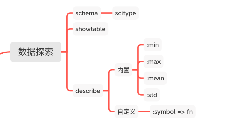
1.1 总览 `showtable`

showtable(X) # 这个大家在jupyter notebook里试一下就好了，我这里不能导出markdown，我让别人帮我试了一下也有问题，那就是作者的问题了

1.2 查看每列的科学类型 `schema`

schema(boston)

_.names	_.types	_.scitypes
Crim	Float64	Continuous
Zn	Float64	Continuous
Indus	Float64	Continuous
Chas	Int64	Count
NOx	Float64	Continuous
Rm	Float64	Continuous
Age	Float64	Continuous
Dis	Float64	Continuous
Rad	Int64	Count
Tax	Int64	Count
PTRatio	Float64	Continuous
Black	Float64	Continuous
⋮	⋮	⋮

注意

1.3 自定义查看内容 `describe`

需要注意的是，describe不能对命名元组起作用，需要DataFrame类型，这个函数是专门为DataFrame设计的

1.3.1 内置功能

describe(X, :nmissing) # 每一列有missing的数量
13×2 DataFrame

Row	variable	nmissing
	Symbol	Nothing
1	Crim
2	Zn
3	Indus
4	Chas
5	NOx
6	Rm
7	Age
8	Dis
9	Rad

describe(X, :min, :max, :mean, :std) # 每一列的最小值，最大值，平均值，标准差，他们会跳过missing

Row	variable	min	max	mean	std
	Symbol	Real	Real	Float64	Float64
1	Crim	0.00632	88.9762	3.61352	8.60155
2	Zn	0.0	100.0	11.3636	23.3225
3	Indus	0.46	27.74	11.1368	6.86035
4	Chas	0	1	0.06917	0.253994
5	NOx	0.385	0.871	0.554695	0.115878
6	Rm	3.561	8.78	6.28463	0.702617
7	Age	2.9	100.0	68.5749	28.1489
8	Dis	1.1296	12.1265	3.79504	2.10571
9	Rad	1	24	9.54941	8.70726
10	Tax	187	711	408.237	168.537
11	PTRatio	12.6	22.0	18.4555	2.16495
12	Black	0.32	396.9	356.674	91.2949
13	LStat	1.73	37.97	12.6531	7.14106

1.3.2 自定义功能

desribe(X, :symbol => fn) # fn作用于整个列

desribe(X, :symbol => sum)

Row	variable	symbol
	Symbol	Real
1	Crim	1828.44
2	Zn	5750.0
3	Indus	5635.21
4	Chas	35
5	NOx	280.676
6	Rm	3180.02
7	Age	34698.9
8	Dis	1920.29
9	Rad	4832
10	Tax	206568
11	PTRatio	9338.5
12	Black	180477.0
13	LStat	6402.45

2. 数据清洗

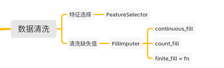
2.1 特征选择 `FeatureSelector`

文档
FeatureSelector(features=Symbol[])
注意
这个model用来选择DataFrame或NamedTuple的特征字段
示例

model = FeatureSelector([:Crim]) # 选择Crim的特征字段
mach = fit!(machine(model, X))
MLJ.transform(mach, X) |> df -> first(df, 5) # 这里的transform会与DataFrame的transform冲突，要指定模块为MLJ

表格太难打了，我这里就给出5个数据好了

Row	Crim
	Float64
1	0.00632
2	0.02731
3	0.02729
4	0.03237
5	0.06905

2.2 清洗缺失值 `FillImputer`

文档

FillImputer(
   features        = [],
   continuous_fill = e -> skipmissing(e) |> median
   count_fill      = e -> skipmissing(e) |> (f -> round(eltype(f), median(f)))
   finite_fill     = e -> skipmissing(e) |> mode)

注意
FillImputer可以指定特征列来填充missing值，默认的填充函数以给出，也可以自己定义

• continuous_fill: function to use on Continuous data, by
default the median
• count_fill: function to use on Count data, by default the
rounded median
• finite_fill: function to use on Multiclass and OrderedFactor
data (including binary data), by default the mode

示例

df = coerce((x1 = 1:3, x2 = [missing, 1, 2]), :x2 => Continuous)
schema(df)

_.name	_.types	_.scitype
x1	Int64	Count
x2	Union{Missing, Float64}	Union{Missing, Continuous}

model = FillImputer(continuous_fill = e -> skipmissing(e) |> mean)
mach = fit!(machine(model, df))
w = MLJ.transform(mach, df)	
schema(w)

julia> w = MLJ.transform(mach, df)
(x1 = 1:3,
 x2 = [1.5, 1.0, 2.0],)

_.name	_.types	_.scitype
x1	Int64	Count
x2	Union{Missing, Float64}	Continuous

3. 数据转换

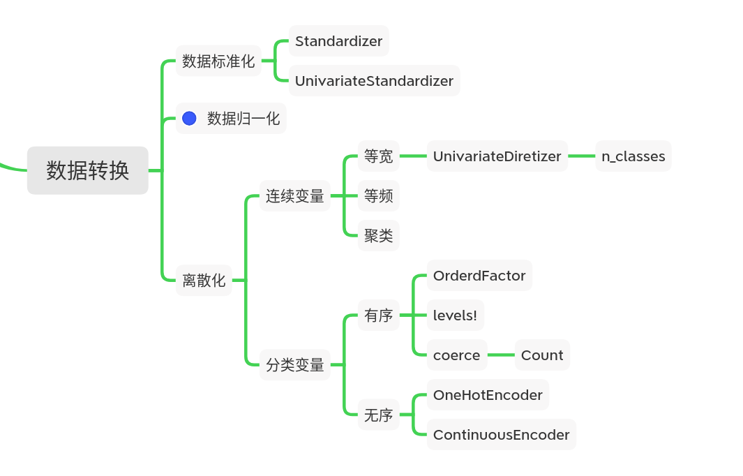
3.1 数据标准化 `Standardizer`

文档
Standardizer(; features=Symbol[], ignore=false, ordered_factor=false, count=false)

newX = \frac{X' - mean(X)} {Std(X)}

注意
其中

X’ 需要转换的数组
X 用来拟合的原数据
newX 转换X’ 后的新数组

另外
Standardizer只对Continuous科学类型的数据有效，如果在数据集中有科学类型为OrderedFactor或Count的nums，可以在Standardizer中指定ordered_factor=true或count=true

示例

X = (ordinal1 = [1, 2, 3],
              ordinal2 = categorical([:x, :y, :x], ordered=true),
              ordinal3 = [10.0, 20.0, 30.0],
              ordinal4 = [-20.0, -30.0, -40.0],
              nominal = categorical(["Your father", "he", "is"]));

schema(X)

_.names	_.types	_.scitypes
ordinal1	Int64	Count
ordinal2	CategoricalArrays.CategoricalValue{Symbol,UInt32}	OrderedFactor{2}
ordinal3	Float64	Continuous
ordinal4	Float64	Continuous
nominal	CategoricalArrays.CategoricalValue{String,UInt32}	Multiclass{3}

尝试先不把ordinal1转换

model = Standardizer()
mach = fit!(machine(model, X))
transform(mach, X)

(ordinal1 = [1, 2, 3],
 ordinal2 = CategoricalArrays.CategoricalValue{Symbol,UInt32}[:x, :y, :x],
 ordinal3 = [-1.0, 0.0, 1.0],
 ordinal4 = [1.0, 0.0, -1.0],
 nominal = CategoricalArrays.CategoricalValue{String,UInt32}["Your father", "he", "is"],)

下面我们将Count和OrderedFactor转换
不过这里需要对ordered_factor=true另外说明
不管这个nums的内容是什么类型，Standardizer都能帮他转换。
不过在此之前先会把nums转化为数字数组

# 先将X的ordinal2提取出来
temp = X.ordered2
nums = coerce(temp, Count)
# 3-element Array{Int64,1}:
#  1
#  2
#  1

model = UnivariateStandardizer() # UnivariateStandardizer 和 Standardizer 类似, UnivariateStandardizer不能用在命名元组DataFrame上，另外UnivariateStandardizer没有参数，不会忽略Count类型
mach = fit!(machine(model, nums)
transform(mach, nums)```

```julia
 -0.5773502691896256
  1.1547005383792517
 -0.5773502691896256

验证一下我们的想法

model = Standardizer(ordered_factor = true)
mach = fit!(machine(model, X))
transform(mach, X)

可以看到ordered2那里一毛一样

(ordinal1 = [-1.0, 0.0, 1.0],
 ordinal2 = [-0.5773502691896256, 1.1547005383792517, -0.5773502691896256],
 ordinal3 = [-1.0, 0.0, 1.0],
 ordinal4 = [1.0, 0.0, -1.0],
 nominal = CategoricalArrays.CategoricalValue{String,UInt32}["Your father", "he", "is"],)

3.2 数据归一化

文档里没有找到，可能要自定义模型了

3.3 数据离散化

连续变量
本来连续变量的离散化分为等宽，等频，聚类等，但是在文档里只找到了等宽离散化的UnivariateDiretizer
文档

  UnivariateDiscretizer(n_classes=512)

  Returns an MLJModel for for discretizing any continuous vector v
  (scitype(v) <: AbstractVector{Continuous}), where n_classes describes
  the resolution of the discretization.

注意
等宽离散化，n_classes代表你想分多少个类
返回值为分类数组OrderedFactor
示例
这里我们对一个1 ~ 100的数组进行等宽离散化，我们把类别设置为10，转换一些随机数

data = coerce(1:100, Continuous)
t = UnivariateDiscretizer(n_classes = 10)
discretizer = fit!(machine(t, data))
v = rand(1:100, 10)
w = transform(discretizer, v)

随机数 v	分类顺序
11	2
54	6
19	2
92	10
43	5
53	6
87	9
23	3
39	4
91	10

tips
用convert(Vector{Int}, w)获得分类数据的排序情况

分类变量

有序变量 OrderedFactor
在文档里没有这个模型，不过作者告诉我可以用coerce强制转换科学类型
如果按原有的分类顺序来转换

nums = categorical([:x, :y:, :z], ordered=true)
levels(nums) # 1, 2, 3
coerce(nums, Count) # 1,2,3
coerce(nums, Continuous) # 1.0 2.0 3.0

也可以改变分类顺序

levels!(nums, [:z, :y, :z])
coerce(nums, Count) # 3, 2, 1

无序变量 Multiclass
文档
有两个模型可以做这个，OneHotEncoder和ContinuousEncoder

  OneHotEncoder(; features=Symbol[],
            ignore=false,
            ordered_factor=true,
            drop_last=false)

  ContinuousEncoder(one_hot_ordered_factors=false, drop_last=false)

注意
两个模型作用一样，在转换的过程中保留Infinite数据，转换Multiclass数据，不过ContinuousEncoder会丢弃无关的数据，如Textual数据，OneHotEncoder会保留所有特征字段

额，他们怎么转换我说不清，看代码把
示例

OneHotEncoder

data = (col = ["a", "b", "c"],)
nums = coerce(data, :col => Multiclass{3})
model = OneHotEncoder()
mach = fit!(machine(model, nums))
transform(mach, nums)

(col__a = [1.0, 0.0, 0.0],
col__b = [0.0, 1.0, 0.0],
col__c = [0.0, 0.0, 1.0],)

ContinuousEncoder

data = (col = ["a", "b", "c"],
vals = [1, 2, 3])
schema(data)

_.names	_.types	_.scitypes
col	String	Textual
vals	Int64	Count

model = ContinuousEncoder()
mach  = fit!(machine(model, data))
transform(mach, data)

(vals = [1.0, 2.0, 3.0],)

详细文档在这里

SHIELD-SKY · 2020 年8 月 26 日 16:10

我自己的数据是matrix，标签也是matrix或者vector。
用data=MLJ.table(data) 好像models(data)是可以搜出一些模型
但是加上label=MLJ.table(label). models(data,label) 就不行了。
不知道各位怎么处理这种基本数据？

nesteiner · 2020 年8 月 27 日 01:16

我记得train_data是一个DataFrame或命名元组，labels是一个数组，他里面没有命名字段，你不应该用models(data, label)

SHIELD-SKY · 2020 年8 月 31 日 02:57

谢谢这个解决了。有个另一个问题，
confusion_matrix(y_hat, y_test)

Warning: The classes are un-ordered,
│ using: negative='0' and positive='1'.
│ To suppress this warning, consider coercing to OrderedFactor.

有什么办法指定negative 和 positive吗？

nesteiner · 2020 年8 月 31 日 07:12

将这些数组的科学类型转为OrderedFactor就行了

nums = categorical([1, 2], ordered = true)
levels(nums) == [1, 2] # true

另外如果想特别指定顺序的话

import CategoricalArrays: CategoricalArray
nums = Categorical([1, 2], levels = [2, 1])
levels(nums) == [2, 1] # true

SHIELD-SKY · 2020 年8 月 31 日 09:05

```
categorical(df::AbstractDataFrame, cols=Union{AbstractString, Missing};
            compress::Bool=false)
```

Return a copy of data frame  `df`  with columns  `cols`  converted to  `CategoricalVector` .

`cols`  can be any column selector ( `Symbol` , string or integer;  `:` ,  `All` ,  `Between` ,  `Not` , a regular expression, or a vector of  `Symbol` s, strings or integers) or a  `Type` .

If  `categorical`  is called with the  `cols`  argument being a  `Type` , then all columns whose element type is a subtype of this type (by default  `Union{AbstractString, Missing}` ) will be converted to categorical.

If the  `compress`  keyword argument is set to  `true`  then the created  `CategoricalVector` s will be compressed.

All created  `CategoricalVector` s are unordered.

**Examples**

```
julia> df = DataFrame(a=[1,2], b=["a","b"])
2×2 DataFrame
│ Row │ a     │ b      │
│     │ Int64 │ String │
├─────┼───────┼────────┤
│ 1   │ 1     │ a      │
│ 2   │ 2     │ b      │

julia> categorical(df)
2×2 DataFrame
│ Row │ a     │ b    │
│     │ Int64 │ Cat… │
├─────┼───────┼──────┤
│ 1   │ 1     │ a    │
│ 2   │ 2     │ b    │

julia> categorical(df, :)
2×2 DataFrame
│ Row │ a    │ b    │
│     │ Cat… │ Cat… │
├─────┼──────┼──────┤
│ 1   │ 1    │ a    │
│ 2   │ 2    │ b    │
```

看了下文档，没有levels 这个参数啊?

nesteiner · 2020 年8 月 31 日 10:01

写错了，我改一下
你再看看

SHIELD-SKY · 2020 年9 月 1 日 02:36

y_test =  categorical(y_test, ordered=true)
levels!(y_test, [1,0])

nesteiner · 2020 年9 月 1 日 02:44

也行，我也这样用好了

SHIELD-SKY · 2020 年9 月 1 日 09:02

ERROR: LoadError: ArgumentError: Expected a matrix of size ≥ 2x2.
Stacktrace:
 [1] MLJBase.ConfusionMatrix(::Array{Int64,2}, ::Array{String,1}) at C:\Users\APTX\.julia\packages\MLJBase\cJmIS\src\measures\confusion_matrix.jl:23
 [2] confusion_matrix(::CategoricalArray{Integer,1,UInt32,Integer,CategoricalValue{Integer,UInt32},Union{}}, ::CategoricalArray{Integer,1,UInt32,Integer,CategoricalValue{Integer,UInt32},Union{}}; rev::Nothing, perm::Nothing, warn::Bool) at C:\Users\APTX\.julia\packages\MLJBase\cJmIS\src\measures\confusion_matrix.jl:109
 [3] confusion_matrix(::CategoricalArray{Integer,1,UInt32,Integer,CategoricalValue{Integer,UInt32},Union{}}, ::CategoricalArray{Integer,1,UInt32,Integer,CategoricalValue{Integer,UInt32},Union{}}) at C:\Users\APTX\.julia\packages\MLJBase\cJmIS\src\measures\confusion_matrix.jl:69

不知道为什么，混淆矩阵时不时的出错

@show size(y_test)
@show size(y_hat)
    
confuma = confusion_matrix(y_hat, y_test)

我这里y_test, y_hat都是
size(y_test) = (100,)
size(y_hat) = (100,)

SHIELD-SKY · 2020 年9 月 1 日 09:02

而且有时候重新再运行一下，这个错就没了

nesteiner · 2020 年9 月 1 日 10:27

你把代码给我吧，我看看
顺便贴下scitype(y_test)和scitype(y_hat)
你也可以更新一下MLJ，我这边的版本是0.12.0

SHIELD-SKY · 2020 年9 月 18 日 08:20

才发现。。两周了。今天用scitype 看了下，发现确实不一致，现在更正了。另外，我在vscode输出confusion_matrix 的时候，不是一个表格的表示方式，请问需要用什么特殊的输出命令才能在vscode中输出图形化的表示吗。repl里

nesteiner · 2020 年9 月 18 日 15:06

vscode没用过诶，都是用Emacs
REPL里显示出来的就是表格

jianlin666 · 2020 年10 月 5 日 15:22

归一化可用 StatsBase.fit 方法
fit(UnitRangeTransform, X; dims=nothing, unit=true)